Scikit-learn Datasets 1: make_classification

I’d like to start a series outlining snippets and patterns relating to machine learning that I’ve found useful.
Many people reading this may already know that that majority of your time working in the realm of data science is spent on data collection and cleaning. Sometimes a good bit is spent on engineering, deployment, monitoring, reporting, and so on. A relatively small fraction is spent on the modeling process itself, so it’s easy for your modeling skills to atrophy. The topic of today’s post is going to be looking at some functions exposed by the sklearn.datasets API that you can use to keep your modeling skills sharp even if modeling hasn’t been your most recent focus.
The goal here is to practice modeling unfamiliar data. By “practice” I mean getting experience in the space between the point where you’ve got a “clean” dataset, up to the point of model deployment. In my experience it’s expected that you can implement this section of a data pipeline fairly quickly from memory, so it’s good to be able to practice it. While there’s a ton of datasets on the internet, typically they’re either the same data sets you’ve seen a million times, and/or they’re not clean datasets that let you jump into modeling. If your goal is to practice modeling, you don’t want to spend all your time doing data collection and/or cleaning! This is where helper functions like make_classification come in handy. There are a number of other helper functions that do similar things (make_blobs and make_gaussian_quantiles are notable examples, but for the purposes of this post I’m just focusing on make_classification).
Basic Usage⌗
For starters, let’s say you want to work on a binary classification problem: 1000 observations, 25 features, and two categories in the target variable. You can generate that pretty trivially:
x, y = make_classification(n_samples=1000, n_features=25, n_classes=2)
With that one line you’re off to the races. You can do your train-test-split, cross validation, feature selection, hyperparameter tuning, model selection, and all that jazz.
A Slightly Deeper Look⌗
Let’s tweak some of the arguments and generate some datasets to see what they do. The first few of these are pretty obvious; for instance, tweaking n_samples changes the number of rows/observations. Unfortunately for this example, altering n_samples seems to affect the randomization of the underlying feature distribution(s), but you should still get the idea:
| n_samples = 100 | n_samples = 1000 |
|---|---|
|
|
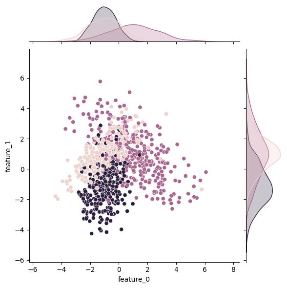
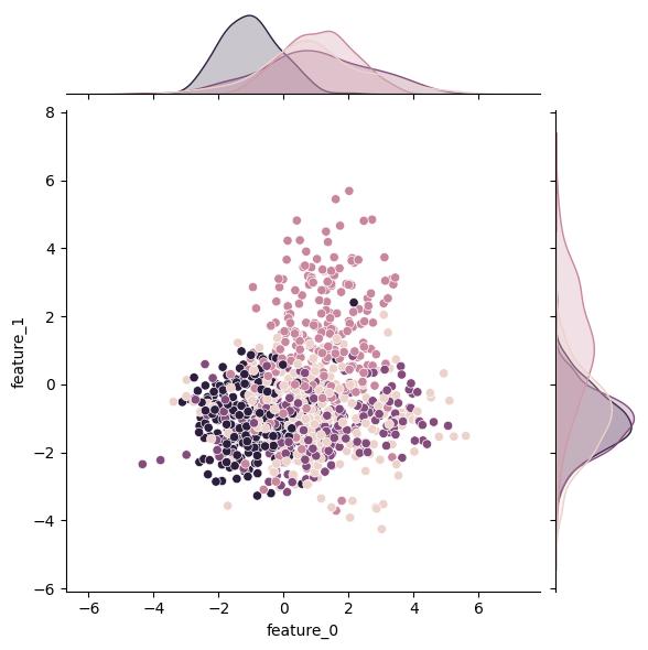
n_classes changes the number of classes in the output (target) variable:
| n_classes = 2 | n_classes = 3 | n_classes = 4 |
|---|---|---|
|
|
|
The real power of this function is the control you have over the information content of the features. Unsurprisingly, n_features lets you adjust the number of features (i.e., columns). More importantly, the n_informative, n_redundant, and n_repeated kwargs control how many and to what extent the features actually affect the output variable.
The docs explain what an “informative” feature is fairly precisely so I’ll just copy it here:
The number of informative features. Each class is composed of a number of
gaussian clusters each located around the vertices of a hypercube in a subspace
of dimension n_informative. For each cluster, informative features are drawn
independently from N(0, 1) and then randomly linearly combined within each
cluster in order to add covariance. The clusters are then placed on the vertices
of the hypercube.
A “redundant” feature is one that’s generated as a linear combination of two informative features. A “repeated” feature is simply drawn randomly from the set of informative and redundant features. The flip_y kwarg is tangentially related; it controls the fraction of samples whose class is assigned randomly (effectively adding noise). The remaining (uninformative) features are drawn at random.
This lets you generate data sets that are more realistic and arguably better suited for practicing certain aspects of your modeling pipeline and/or problem domains. You can easily generate datasets with hundreds of features, many of which may exhibit degeneracy and/or co-linearity with other features. You can generate balanced or highly imbalanced data sets. Since you’re effectively blind, this is also a great way to practice the feature selection aspect of your modeling. This is a great way to get comfortable letting the the data drive your decisions, rather than relying strictly on your priors.
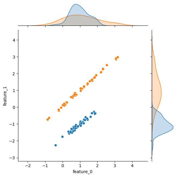
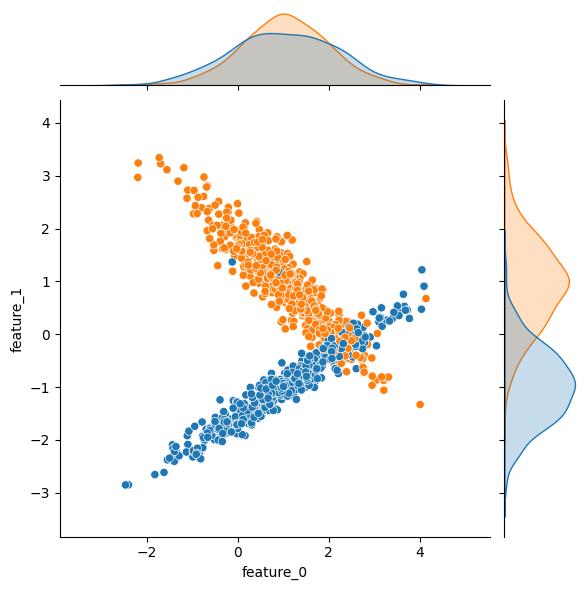
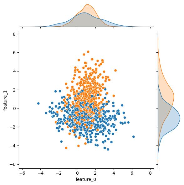
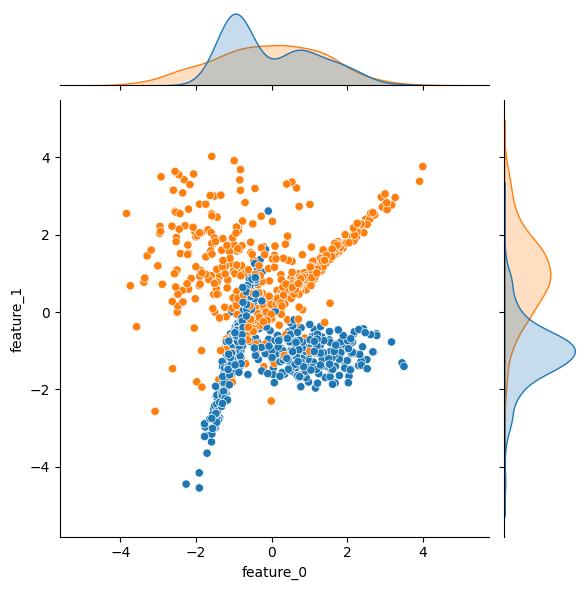
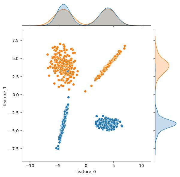
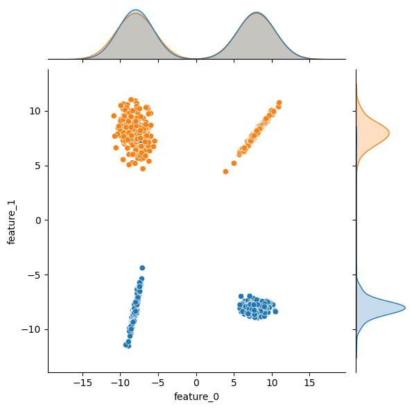
Moving through API, the n_clusters_per_class kwarg sets the number of clusters per class. The class_sep, shift, and scale kwargs can be leveraged to transform the clusters. As an example, here are some plots showing the effect increasing the class_sep value. As an additional bonus, the effect of n_clusters_per_class = 2 is readily apparent in these example plots; both the blue and the orange output classes have two distinct clusters in this feature space.
| class_sep = 1 | class_sep = 4 | class_sep = 8 |
|---|---|---|
|
|
|
The weights kwarg controls the relative population size of the resulting classes. By default classes are balanced, but if your problem domain relates to anomaly detection and/or fraud type problems, you can create highly imbalanced datasets with this kwarg. There is some potentially unintuitive behavior with this kwarg though, so be sure to read the docs.
| weights = [0.50] | weights = [0.99] | |
|---|---|---|

|
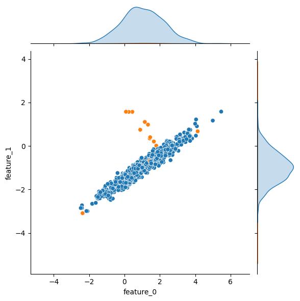
|
Note that if you’re interested in this as a feature exploration exercise, you’ll want to set shuffle to True. Otherwise, the “useful” features are predictably ordered in the the feature matrix:
Without shuffling, X horizontally stacks features in the following order: the
primary n_informative features, followed by n_redundant linear combinations of
the informative features, followed by n_repeated duplicates, drawn randomly with
replacement from the informative and redundant features. The remaining features
are filled with random noise. Thus, without shuffling, all useful features are
contained in the columns X[:, :n_informative + n_redundant + n_repeated].
As I mentioned at the start, there are a number of other similar helper functions to check out that are well suited for other problem domains (e.g., regression). I’ll likely address some of these in a future blog post, but until then, happy hacking!